Edge detection explained in 1D

Written by Akshay Chavan on #arccoder Blog

15 Jan 2017

This post is inspired after watching edge detection (2A-L5,2A-L6) related lectures in the Introduction to Computer Vision course on Udacity. Here I have implemented the real world example shown in the using a 1D toy example.

Edges are the most basic and widely used features used in computer vision. Edges are formed when there is a steep change in the color or intensiy values in the image. To capture these high differnce ridges we can make use of differential opeartors to create masks that computer gradients.

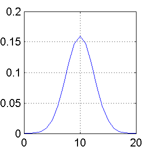
Real world images or signals are never completelty noise free so first we need to smooth the signal using a low pass filter. In this case we have choosen a gausian filter as shown in Fig 1. (This post only implements 1D signal but the same logic can be extended to 2D signals.)

filter

Fig 1: Gaussian filter

Because filtering or convolution is a linear operator, using the associative property of linear operators we can take derivatives of the filter and apply it directly to the signal rather than taking the derivative of the convolved signal and the filter.

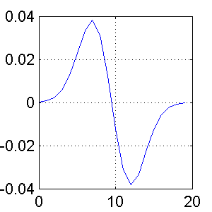
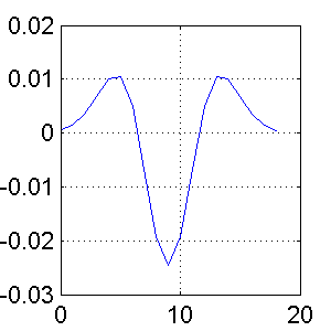
Fig 2 shows the first derivative of the gaussian filter and the second derivative is shown in Fig 3.

dfilter

Fig 2: First derivative of a gaussian filter

d2filter

Fig 3: Second derivative of a gaussian filter

The first order derivative will give the signal which peaks at the location of the largest gradient. But then we need to find the location of the peak to get the edge location. For that we can take another derivative and the location at which the signal crosses over zero thats the location of the peak.

No we apply the filters to the signal shown in Fig 4 with some noise added to it.

signal